Content

• Theory
• 0. structural optimization, kpt convergence, ecut convergence, smearing convergence
• 1. scf
• 2. nscf
• 3. use calculation = 'bands'
• 4. bands.x post-processing
  • bands.x
• 5. plotband.x
• 6. gnuplot
• 7. Python Plotting
• 8. Fatband
  • projwfc.x
  • Suggestion
  • _bands.dat.proj
  • plotband.x
  • further analysis

Band structure refers to the electronic band structure in solid state physics. In general, band structure is the k-E (or k-$\omega$) relation of the electrons distrbuting in crystaline, periodic systems. By analyzing band structure, electronic properties such as

• band gap and its type (direct or indirect), high symmetry points
• phase velocity ($v_{phase}=\frac{\omega}{k}$)
• group velocity ($v_{group}=\frac{d\omega}{dk}$)
• Fermi velocity
• effective mass of charge carriers

Theory

Updating…

The following is an example of the band structure calculation for 4H-SiC bulk crystal in 1x1x1 unit cell.

Example: 4H-SiC crystal, typical wide-bandgap semiconductor, usually for high-power electronics, substrate in semiconductor industry.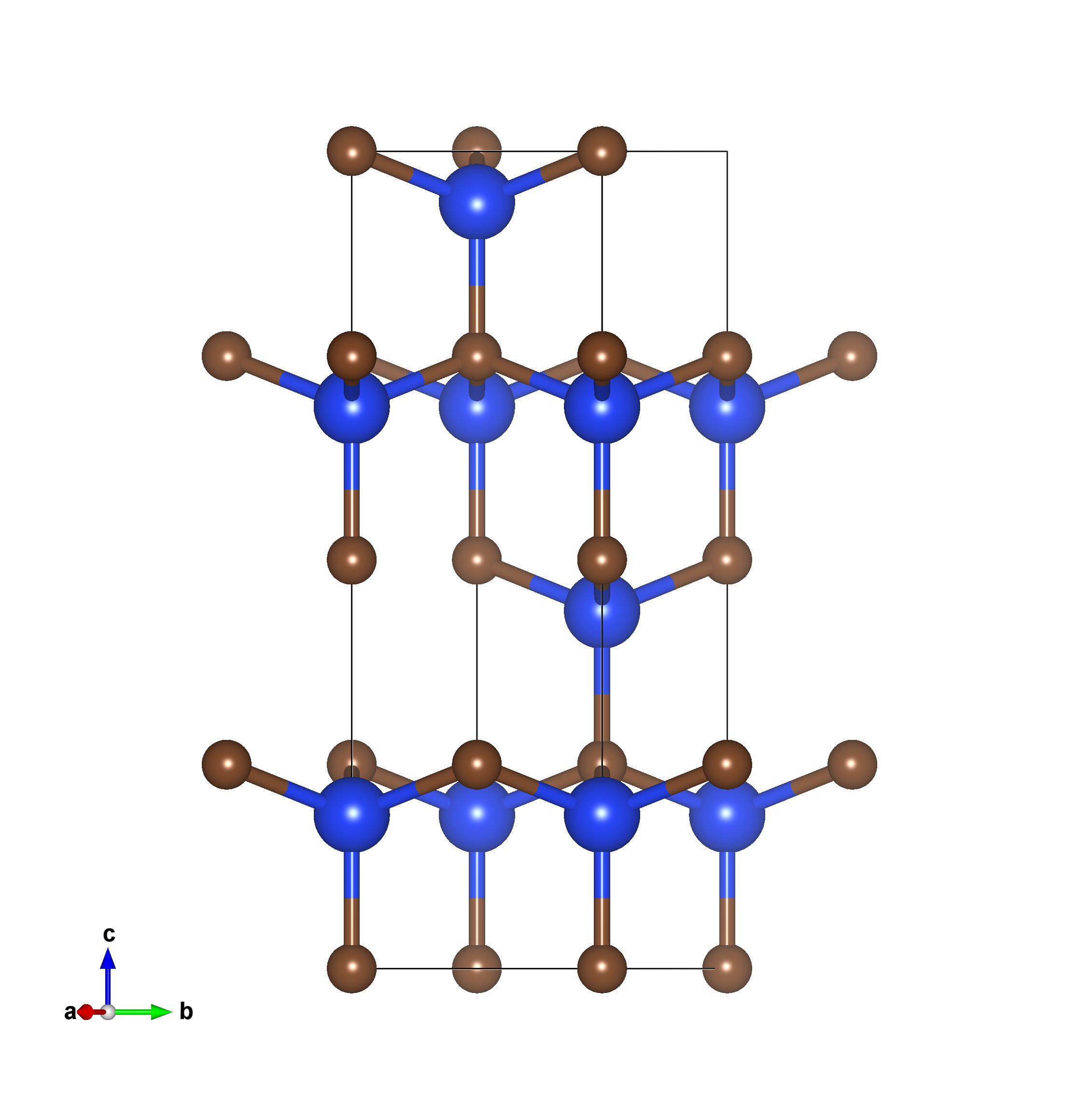

0. structural optimization, kpt convergence, ecut convergence, smearing convergence

Do before any calculation

1. scf

Dense enough K pt mesh

&CONTROL
  title = '4H-SiC'
  prefix = '4HSiC'
  outdir = './calout'
  pseudo_dir = '/home/yongnanli08/Desktop/4hsic/PP'
  calculation = 'scf'
  nstep = 1000
  iprint = 1                ! write band information each iprint step
  tprnfor = .true.          ! calculation of force
  tstress = .true.
  restart_mode = 'from_scratch'
  verbosity = 'high'
  forc_conv_thr = 1e-5      ! no need if not relax vc-relax
  etot_conv_thr = 1e-6      ! no need if not relax vc-relax
/
 
&SYSTEM
  nat= 8
  ntyp= 2
  ibrav= 0
  ecutwfc = 90.00
  nosym = .true.            ! no need, use for low-symmetric system (low-dimensional, etc)
  force_symmorphic = .true. ! no need, force the symmetry group to be symmorphic, for yambo init
  ! =========== Smearing ===============
  occupations = 'smearing'
  smearing = 'mp'
  degauss = 1e-3
/
 
&ELECTRONS
  electron_maxstep = 500
  mixing_mode = 'plain'
  mixing_beta = 0.4
  mixing_ndim = 12
  conv_thr =  1.0d-11
  diagonalization = 'david'
  diago_thr_init = 5e-6     ! for charge density, 1e-5, can reduce if not converged
/
 
&IONS
  ion_dynamics = 'bfgs'     ! for structural optimization, relax & vc-relax
/
 
&CELL
  cell_dynamics = 'bfgs'    ! for structural optimization, relax & vc-relax
/
 
ATOMIC_SPECIES
Si  28.085  Si.pbe-n-rrkjus_psl.1.0.0.UPF
C   12.011  C.pbe-n-kjpaw_psl.1.0.0.UPF
 
CELL_PARAMETERS angstrom
   3.099315860  -0.000000000   0.000000000
  -1.549657930   2.684086271   0.000000000
   0.000000000   0.000000000  10.114801588

ATOMIC_POSITIONS angstrom
Si            1.5496594817        0.8946945267        9.4877890025
Si           -0.0000015518        1.7893917439        4.4303882085
Si            0.0000000000       -0.0000000000        6.9598048955
Si            0.0000000000        0.0000000000        1.9024041015
C             1.5496594817        0.8946945267        7.5821765481
C            -0.0000015518        1.7893917439        2.5247757541
C             0.0000000000        0.0000000000        5.0603888110
C             0.0000000000       -0.0000000000        0.0029880170
 
K_POINTS automatic
8 8 8  0 0 0

2. nscf

actually no need (bands calculation is also nscf), the charge density has been determined in scf

• calculation = 'scf' to calculation = 'nscf'
• k pt 8 8 8 to 16 16 16

3. use calculation = 'bands'

K_POINTS crystal_b
4 ! num_of_high_symmetry_points
0.0000000000	0.0000000000	0.0000000000 30 ! Gamma
0.5000000000	0.0000000000	0.0000000000 20 ! M
0.3333333333	0.3333333333	0.0000000000 30 ! K
0.0000000000	0.0000000000	0.0000000000 20 ! Gamma

The numbers following the coordinates are, the point interval between this high symm. point to the next one while doing interpolating. High symmetry path can check by upload bulk pwscf input file to seekpath. High symmetry point coordinates are in reduced form, in reduced first Brillouin zone!

Can also use Python script KptPath with K_POINTS crystal, same function with K_POINTS crystal_b.

4. bands.x post-processing

bands.x

&BANDS
  prefix = ''
  outdir = ''
  filband = '_bands.dat'
/

will get

• _bands.dat
• _bands.dat.gnu
• _bands.dat.rap

Run (I prefer to call this as a postprocessing opeartion, so with pp), can mpirun

bands.x < .ppbands.in > ppbands..out

5. plotband.x

don’t trust its output of high-symmetry point: , it is in cartesian coordinates, but we want high symm. point in crystal/reduced coordinates!

> plotband.x
     Input file
> 4HSiCslabC_bands.dat
Reading   24 bands at     71 k-points
Range:  -13.9960    7.1910eV  Emin, Emax, [firstk, lastk]
> -6,8
high-symmetry point:  0.0000 0.0000 0.0000   x coordinate   0.0000
high-symmetry point:  0.5000 0.2887 0.0000   x coordinate   0.5774
high-symmetry point:  0.3333 0.5774 0.0000   x coordinate   0.9107
high-symmetry point:  0.0000 0.0000 0.0000   x coordinate   1.5773
output file (gnuplot/xmgr)
> gnuplot
bands in gnuplot/xmgr format written to file gnuplot

output file (ps)
> (press enter)
stopping ...

generate several gnuplot files, splited by high-symmetry points

6. gnuplot

gnuplot -p -e "plot 'gnuplot.1.1' w l, 'gnuplot.2.1' w l, 'gnuplot.3.1' w l, [0:1.5773] 3.8937 w l t 'Fermi level'"

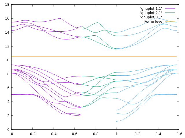
Obviously an indirect band gap is found, between Gamma point as VBM and K point as CBM.

BEAWARE: the use of plotbands.x may introduce some numerical error in post-processing, use

gnuplot -p -e "plot 'prefix_bands.gnu' w l, [0:1.5773] 3.8937 w l t 'Fermi level'"

is better, and then split the band by k point path by yourself (can see plotbands.x ‘s output to know the x coordinate of each high sym. point).

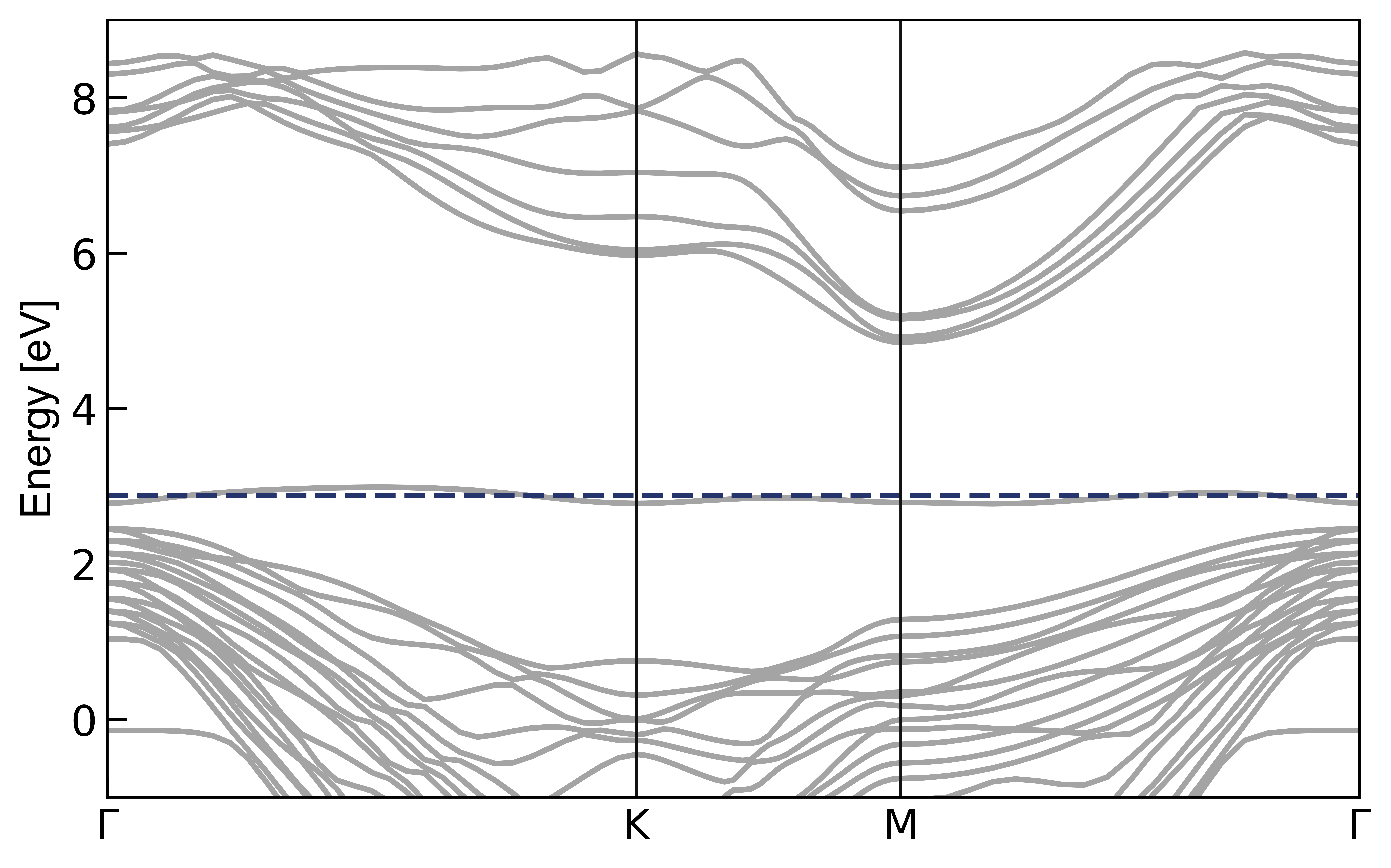
7. Python Plotting

use Bandstructure

8. Fatband

Characteristics of band in our interested-area, and to see which of them are highly hybridized. This analysis called ‘Fatband analysis’. To do this, need to project the atomic orbitals to the Bloch wavefunction and then plot band structure. In simple words, to see the fractional contribution of atomic orbitals to the band structure.

After doing bands.x postprocessing, do another projwfc.x wavefunction projection:

projwfc.x

&projwfc
  prefix = ''
  outdir = './calout'
  DeltaE = 0.01
  filpdos = './PDOS/_pdos.dat'
  filproj = './PROJ/_bands.dat'
  lsym = .false. ! symmetrized
  lwrite_overlaps = .false. ! output of overlap matrix of atomic orbitals, in xml
  kresolveddos = .false. ! k resolved DOS
  tdosinboxes = .false. ! local DOS integrated in volumes
  plotboxes = .false. ! Boxes in xsf format
/

Suggestion

Recommend to create a directory ./PROJ and /PDOS to store the output files, can do the similar thing in bands.x:

  filband = './PROJ/_bands.dat'

and then run, can mpirun, faster

projwfc.x < .projwfc.in > projwfc..out

Be aware here no PDOS output, get output files

• _bands.dat.projwfc_up

change the name from

• _bands.dat.projwfc_up

to

• _bands.dat.proj

the purpose is to let plotband.x recognise the total part and projected parts of bands structures are generated.

_bands.dat.proj

file look like this

      27      27     250      27      27     250       2       1
     0  4.66028467  0.00000000  0.00000000  0.00000000  0.00000000  0.00000000
   1.0000000000000000        4.0549585695515991E-010  -0.0000000000000000     
 -0.49999999959450403       0.86602539062103212        0.0000000000000000     
  -1.6219834278206396E-009  -4.0549585695515991E-010   9.3264047099686778     
      176.0415294730        4.0000000000       80.0000000000     9
   1   C     4.00
   1       0.000000000    0.000000000    0.000000000    1
   2      -0.000000001    0.577350239    0.000000000    1
       8     251      10
    F    F
    1    1  C   2S     1    0    1
       1       1        0.4920425600
       1       2        0.0000000000
       1       3        0.0000000000
       1       4        0.0000000000
       1       5        0.0030914953
       1       6        0.0000000035
       1       7        0.0006870343
       1       8        0.0000000217
       1       9        0.0008474838
       1      10        0.0000001068
       2       1        0.4918940160
       2       2        0.0000000001
       2       3        0.0000867961
       2       4        0.0000000266
       2       5        0.0030785331
       2       6        0.0000000001
       2       7        0.0006861789
       2       8        0.0000000010
       2       9        0.0008435850
       2      10        0.0000000231
       ...

` 8 251 10` represent to

• norbitals
• npkt
• nbnd

` 1 1 C 2S 1 0 1` represent

• orbital index
• atom index
• atom type
• orbital name (principle quantum number n)
• Not sure
• Azimuthal quantum number (0 for s, 1 for p, etc)
• Magnetic quantum number (for p, have px, py, pz)

Can check like this

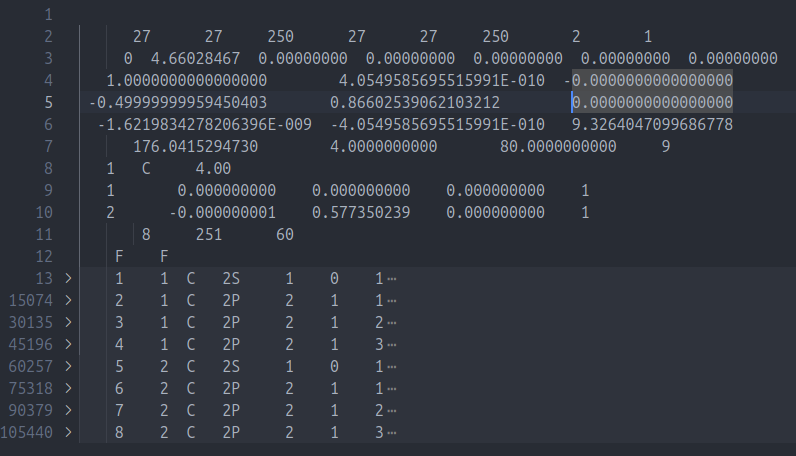
For graphene, as example, one carbon atom have

• one 2s orbital
• three 2p orbitals

And total two carbon atoms, so it can be found that

• 1 1 C 2S
• 2 1 C 2P
• 3 1 C 2P
• 4 1 C 2P
• 5 2 C 2S
• 6 2 C 2P
• 7 2 C 2P
• 8 2 C 2P

plotband.x

Similar to simple plotband.x, but the projected file makes some difference

Remember to go into ./PROJ/ if you created and stored _bands.dat and _bands.dat.proj into

plotband.x
     Input file 
_bands.dat
Reading   10 bands at    251 k-points
List of atomic wavefunctions:
1 4
Range:  -23.7690   10.4000eV  Emin, Emax, [firstk, lastk]
-25,12
high-symmetry point:  0.0000 0.0000 0.0000   x coordinate   0.0000
high-symmetry point:  0.3333 0.5774 0.0000   x coordinate   0.6667
high-symmetry point:  0.5000 0.2887 0.0000   x coordinate   1.0000
high-symmetry point:  0.0000 0.0000 0.0000   x coordinate   1.5774
output file (gnuplot/xmgr) > gnuplot
bands in gnuplot/xmgr format written to file:
gnuplot
output file (ps)
ps
Efermi
-3.3674
deltaE, reference E (for tics)
5 -3.3674
bands in PostScript format written to file: ps
output file for projected band (gnuplot script)
gnuplotscript
run "gnuplot gnuplotscript" to get "gnuplotscript_projected.ps"
and/or run "ps2pdf gnuplotscript_projected.ps" to get "gnuplotscript_projected.pdf"

Files not useful (can delete):

• gnuplot x.x
• ps

Additional setting compared to simple band structure:

• List of atomic wavefunctions:
  • orbital index in _bands.dat.proj
  • here picked the two 2S orbitals (1,4, can be found in _bands.dat.proj)
• Efermi
  • Fermi energy from nscf.out
• deltaE, reference E (for tics)
  • tics interval in plotting
  • reference usually pick Fermi energy again
• output file for projected band (gnuplot script)
  • the code will generate a gnuplot script for plotting, look like

#!gnuplot
set terminal postscript portrait  enhanced color dashed lw 1 ",12"
set output "gnuplotscript_projected.ps"
set xrange [0.0:    1.5774]
unset xtics
#set yrange [  -25.000000:   12.000000]
set ytics   -25.000000,    5.000000,   12.000000 
set ylabel "E - E_{ref} (eV)"
set border lw 0.5
set style arrow 1 nohead front lw 0.5 lc rgb 'black'
set arrow from     0.0000,graph 0 to     0.0000,graph 1 as 1
set arrow from     0.6667,graph 0 to     0.6667,graph 1 as 1
set arrow from     1.0000,graph 0 to     1.0000,graph 1 as 1
set title 'gnuplotscript_projected' noenhanced
plot 'gnuplot' u 1:($2 -    -3.367400):3 w l palette lw 1 notitle, \
    0.000000 lt 2 lw 0.5 lc rgb 'grey50' notitle

Comment out the first line set terminal ...

then gnuplot -p gnuplotscript will show up a gnuplot window and a .ps file gnuplotscript_projected.ps

and then ps2pdf gnuplotscript_projected.ps will convert the .ps file to a pdf one

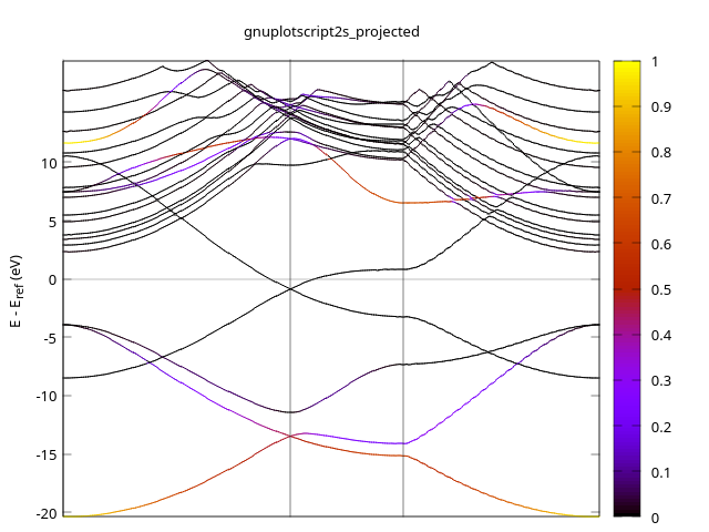
Can see the 2S orbitals contribute less (or even no contribution) near Fermi level

further analysis

can be done by inspect the contribution of others orbitals, by changing List of atomic wavefunctions: in plotband.x

can use the following codes for faster plotting (graphene case):

plotband.x input (2s for example)

mono_ppbands.dat
1 5
-25 12
gnuplot2s
ps
-3.3674
5 -3.3674
gnuplotscript2s

run.sh

#!/bin/sh

for i in 2s 2p1 2p2 2p3;do
	plotband.x < ppband${i}.in > out.ppband${i}
	sed -i '2s/^/#/' gnuplotscript${i}
	gnuplot -p gnuplotscript${i}
done

rm gnuplot*.1
rm ps

• 2S

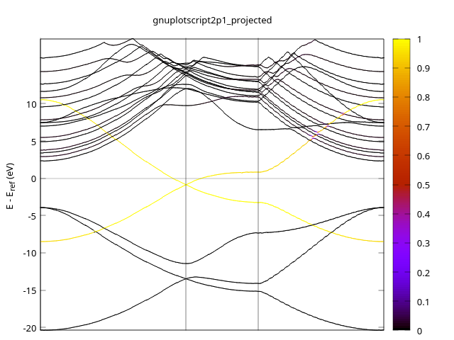
• 2P1

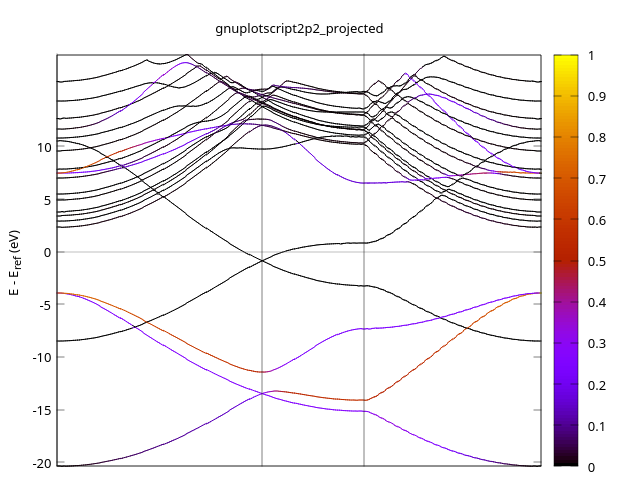
• 2P2

• 2P3

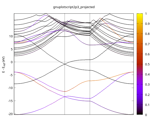
By this it is clear that the atomic orbital in graphene should be sp2 hybridization + pz (2p1 here), in which pz contribute the most to the states near Fermi level