Yambo for Linear Optics responses
Published:
Content
- Theory
- 0. scf (or nscf)
- 1. Yambo initialization
- 2. Yambo linear optics
- 3. Output files
- 4. Convergence
Optical responses of materials can be computed based on linear response theory, in which considering the electron density response of system to the external electric field. This is linked to the electric displacement field and the polarization field in Maxwell equations:
\[\vec D(\omega)=\varepsilon_0 \varepsilon_r(\omega) \vec E(\omega)=\varepsilon_0 (1+\chi) \vec E\]in which \(\varepsilon_r=1+\chi\) is the relative dielectric constant, and \(\chi\) is the electric susceptibility, defining the polarization field \(\vec P=\chi \vec E\)
For simply, use \(\varepsilon(\omega)=1+\chi(\omega)\) as relative dielectric function, considering its spectral dispersion.
Theory
In short, the (reversed) dielectric function is the response function of the external field. Or, the electrical susceptibility is response function. The generalized form of the definition of response function \(\chi(t)\) is
\[F(t)=\int_0^{\infty} \chi(\tau) g(t-\tau) d\tau\]In electric field expression, it is
\[V_{scattering}(\vec r,t)=V_{ext}(\vec r,t)+V_{ind}(\vec r,t)\] \[V_{scattering}(\vec r,\omega)=\int d\vec r' \varepsilon_{nn}^{-1}(\vec r, \vec r', \omega)V_{ext}(\vec r,\omega)\]Updating…
For Yambo calculation, a prelinminary SCF (or NSCF) calculation of the electron density distribution is needed. Below takes QE PWscf as example
0. scf (or nscf)
go to output file, go prefix.save folder, type p2y (pwscf to yambo for memorizing). Generating folder SAVE.
create directory yambo at anywhere, and copy SAVE to that directory.
1. Yambo initialization
just type yambo in the shell, the code will detect the SAVE folder and generate a r_setup file, with information of the system:
      __   __     _        __  __       ____      U  ___  u
      \ \ / / U  /"\  U u |" \/ "| u U | __") u    \/"_ \/
       \ V /   \/ _ \/   \| |\/| |/   \|  _ \/     | | | |
      U_|"|_u  / ___ \    | |  | |     | |_) | .-,_| |_| |
        |_|   /_/   \_\   |_|  |_|     |____/   \_)-\___/
    .-,//|(_   \\    >>  <<,-,,-.     _|| \\_        \\
     \_) (__) (__)  (__)  (./  \.)   (__) (__)      (__)


    Version 5.2.1 Revision 22792 Hash (prev commit) ace55e496e
                           Branch is
                MPI+SLK+SLEPC+HDF5_MPI_IO Build
                   http://www.yambo-code.org

 12/23/2024 at 15:39 yambo @ ln201
 ==================================================
...
 [RD./SAVE//ns.db1]--------------------------------------------------------------
  Bands                                            :   8
  K-points                                         :   450
  G-vectors                                        :   78781 [RL space]
  Components                                       :   9969 [wavefunctions]
  Symmetries                                       :  2 [spatial+T-reV]
  Spinor components                                :  1
  Spin polarizations                               :  1
  Temperature                                      :  0.025852 [eV]
  Electrons                                        :  8.000000
  WF G-vectors                                     :  14401
  Max atoms/species                                :  2
  No. of atom species                              :  1
  Exact exchange fraction in XC                    :  0.000000
  Exact exchange screening in XC                   :  0.000000
  Magnetic symmetries                              : no
 - S/N 001656 ---------------------------------------------- v.05.02.01 r.22792 -
...
  [02.03] Reciprocal space
  ========================

  nG shells         :   4072
  nG charge         :   78781
  nG WFs            :  14437
  nC WFs            :   9973
...
  [02.04] K-grid lattice
  ======================

  Compatible Grid is   : 2D
  Base K vectors       :  K_min[ 1 ]  K_min[ 2 ]  K_min[ 3 ]
  K_min[ 1 ] : -0.34694E-17 -0.33333E-01   0.0000     [rlu]
  K_min[ 2 ] :  0.33333E-01  0.69389E-17   0.0000     [rlu]
  Grid dimensions      :  30  30
  K lattice UC volume  :  0.337683E-3 [a.u.]

  IBZ K-points :   450
  BZ  K-points :   900
...
  [02.05] Energies & Occupations
  ==============================

  [X] === General ===
  [X] Electronic Temperature                        :  0.258606E-1   300.100    [eV K]
  [X] Bosonic    Temperature                        :  0.258606E-1   300.100    [eV K]
  [X] Finite Temperature mode                       : yes
  [X] El. density                                   :  0.66145E+23 [cm-3]
  [X] Fermi Level                                   : -4.235844 [eV]

  [X] === Gaps and Widths ===
  [X] Conduction Band Min                           : -4.235844 [eV]
  [X] Valence Band Max                              : -4.235844 [eV]
  [X] Filled Bands                                  :   4
  [X] Metallic Bands                                :   5   5
  [X] Empty Bands                                   :   6   8

  [X] === Metallic Characters ===
  [X] N of el / N of met el                         :   8.00000     0.257934E-6
  [X] Average metallic occ.                         :  0.644836E-7
can find information such as
- number of bands
- number of G-vectors wavefunctions (nG WFs)
- corresponding temperature (Fermi-Dirac in electrons)
- electron density
- Fermi level
- CBM, VBM, Bandgap, Filled & Empty bands
in this case is graphene, so a metallic system is assumed.
Each input file of Yambo code can be generated by the code itself. Only need to change some parameters in the input file.
2. Yambo linear optics
can be IP (independent particle) and RPA (random phase approximation), the difference is the input command.
For IP
yambo -o c -F ip.in
For RPA
yambo -o c -k hartree -V RL -F rpa.in
get input file rpa.in as
optics                           # [R] Linear Response optical properties
kernel                           # [R] Kernel
rim_cut                          # [R] Coulomb potential
chi                              # [R][CHI] Dyson equation for Chi.
dipoles                          # [R] Oscillator strenghts (or dipoles)
FFTGvecs= 14451            RL    # [FFT] Plane-waves
Chimod= "HARTREE"                # [X] IP/Hartree/ALDA/LRC/PF/BSfxc
NGsBlkXd=  4               Ry    # [Xd] Response block size
% QpntsRXd
 1 | 1 |                             # [Xd] Transferred momenta
%
% BndsRnXd
  1 |  8 |                           # [Xd] Polarization function bands
%
% EnRngeXd
  0.00000 | 10.00000 |         eV    # [Xd] Energy range
%
% DmRngeXd
 0.100000 | 0.100000 |         eV    # [Xd] Damping range
%
ETStpsXd= 1001                   # [Xd] Total Energy steps
% LongDrXd
 1.000000 | 1.000000 | 0.000000 |        # [Xd] [cc] Electric Field
%
| -o | optics |
| c :linear optics | |
| -k | kernel |
| hartree: for RPA | |
| -F | file |
usually with -V RL, -V for verbosity (advanced setting), -V RL generate the line
FFTGvecs= 14451 RL # [FFT] Plane-waves
is the FFT cutoff, corresponds to PWscf ecutwfc.
To run Yambo, just type
yambo -F rpa.in -J RPA
where -J RPA refers to the job name, creating folder RPA to save temporary files. All of the output files will be at the same directory of SAVE if the job name is assigned (no job name is needed and only -F is ok for somecases, to save files in SAVE directly).
3. Output files
check the following before run
% QpntsRXd
 1 | 1 |                             # [Xd] Transferred momenta
%
% BndsRnXd
  1 |  8 |                           # [Xd] Polarization function bands
%
% EnRngeXd
  0.00000 | 10.00000 |         eV    # [Xd] Energy range
%
% DmRngeXd
 0.100000 | 0.100000 |         eV    # [Xd] Damping range
%
ETStpsXd= 1001                   # [Xd] Total Energy steps
% LongDrXd
 1.000000 | 0.000000 | 0.000000 |        # [Xd] [cc] Electric Field
%
| QpntsRXd | q point, macroscopic use 1,1 ok |
| BndsRnXd | bands, include as much as possible, usually around bandgap |
| EnRngeXd | Energy range of output |
| DmRngeXd | Damping, usually is ok to default |
| ETStpsXd | Energy step, for 10eV length I like 1001 |
| LongDrXd | Response direction, cartersian direction |
output log
usually start with r-jobname-.... as, containing same information as r_setup
...
 Timing [Min/Max/Average]: 01m-56s/01m-56s/01m-56s

 [06] Dipoles
 ============

 [RD./SAVE//ns.kb_pp_pwscf]------------------------------------------------------
  Fragmentation                                    : yes
 - S/N 004183 ---------------------------------------------- v.05.02.01 r.22792 -
 [WF-Oscillators/G space/Transverse up loader] Normalization (few states)  min/max  :  0.10955E-15   1.0000

 [WR./RPA110//ndb.dipoles]-------------------------------------------------------
  Brillouin Zone Q/K grids (IBZ/BZ)                :   1802   3600   1800   3600
  RL vectors                                       :  14451 [WF]
  Fragmentation                                    : yes
  Electronic Temperature                           :  300.1000 [K]
  Bosonic    Temperature                           :  300.1000 [K]
  DIP band range                                   :   1   8
  DIP band range limits                            :   5   5
  DIP e/h energy range                             : -1.000000 -1.000000 [eV]
  RL vectors in the sum                            :  14451
  [r,Vnl] included                                 : yes
  Bands ordered                                    : yes
  Direct v evaluation                              : no
  Approach used                                    : G-space v
  Dipoles computed                                 : R V P
  Wavefunctions                                    : Perdew, Burke & Ernzerhof(X)+Perdew, Burke & Ernzerhof(C)
 - S/N 004183 ---------------------------------------------- v.05.02.01 r.22792 -
...
o-jobname.eps o-jobname.eels
all output file starts with o-jobname
# Absorption @ Q(1):   1.00000000      0.00000000      0.00000000    [q->0 direction]
#
# [ X ] Hartree size                              :  131
# [GEN] GF Energies                               : Perdew, Burke & Ernzerhof(X)+Perdew, Burke & Ernzerhof(C)
# [GEN] Green`s Function                          : Retarded
#
# [GEN] Gauge                                     : Length
# [GEN] [r,Vnl] included                          : yes
#
#    E[1] [eV]          Im(eps)            Re(eps)            Im(eps_o)          Re(eps_o)
#
        0.000000           0.37292E-24        1.000001           0.16273E-17        7.150296
        0.010000           0.170461E-7        1.000001           0.071166           7.152400
        0.020000           0.342534E-7        1.000001           0.143004           7.158704
        0.030000           0.517863E-7        1.000001           0.216202           7.169186
        0.040000           0.698156E-7        1.000001           0.291472           7.183804
...
| RPA | ||||
|---|---|---|---|---|
| Energy | Im(eps) RPA | Re(eps) RPA | Im(eps) IP | Re(eps) IP |
usually contains results at lower level approximation.
4. Convergence
the unit RL is the number of wavefunctions/vectors
FFTGvecs
Always check if FFTGvecs= appears in input file, sometimes disappears even with -V RL. Usually slightly lower than ecutwfc used in scf calculation is ok, just change the unit like
FFTGvecs=60 Ry
60 Ry is almost ok for ecutwfc=80 Ry in scf.
can be check nG WFs in r_setup and r-jobname by finding
  [02.03] Reciprocal space
  ========================
  nG WFs            :  14437
IP
no convergence need except FFTGvecs, also the lowest level of approximation, should be large deviations.
RPA
only parameters added
Chimod= "HARTREE"                # [X] IP/Hartree/ALDA/LRC/PF/BSfxc
NGsBlkXd=  4               Ry    # [Xd] Response block size
| NGsBlkXd | how many Gvecs need to calculate reponse, can start from ~3Ry to test |
can be check in o-jobname by finding
# [ X ] Hartree size : 131
in RL
low dimensional case (with -r)
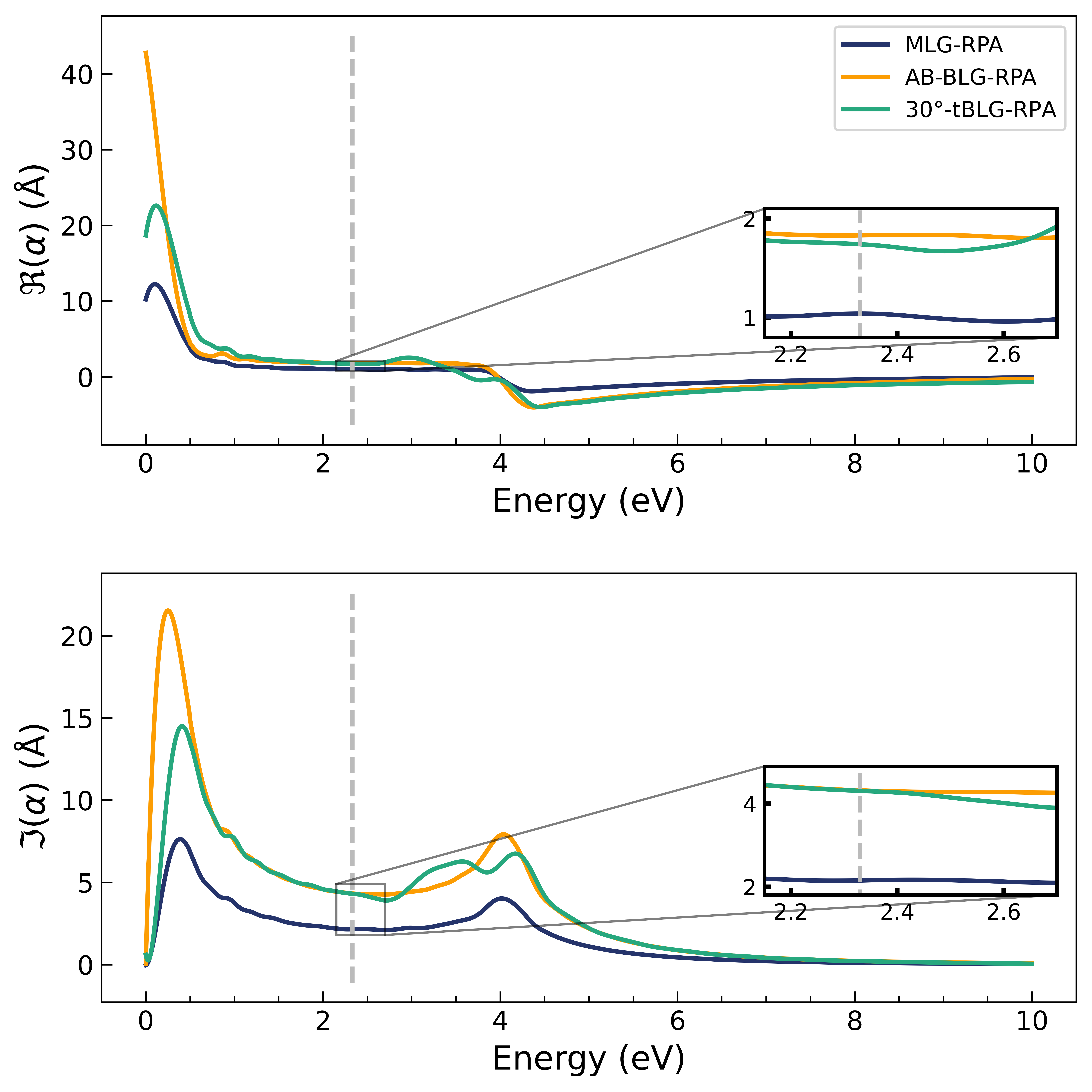
If low dimensional system is used (with -r), Yambo will generate new output file o-jobname.alpha, and o-jobname.eps is useless. In such cases, direct epsilon output will be something like full of vacuum, that is, Im(eps) ~ 0 and Re(eps) ~ 1. It is normal and all of the dielectric information is enbodied in polarizability file o-jobname.alpha instead. Polarizability is defined as (2D materials)
See more in YamboLowD
Below is the polarizability of monolayer graphene and bilayer graphene as demonstration. 


Leave a Comment