QE PWscf Energy Barrier
Published:
Content
- Atomic Modeling
- 0. structural optimization, kpt convergence, ecut convergence, smearing convergence
- 1. NEB
- 2. CI-NEB
- 3. Migration Energy Barrier
- Reference can take a look:
Atomic Modeling
See SlabModeling for slab modeling
Here how to get unit cell with specific crystal orientation is introduced, by Atomsk.
For example, a Cu (111) model is required.
can call Atomsk by command directly
atomsk --create fcc 3.636155 Cu orient [-110] [-1-12] [111] -duplicate 2 2 2 vesta
can also call atomsk first, and get into interactive command line mode
> atomsk
 ___________________________________________________
|              ___________                          |
|     o---o    A T O M S K                          |
|    o---o|    Version Beta 0.13.1                  |
|    |   |o    (C) 2010 Pierre Hirel                |
|    o---o     https://atomsk.univ-lille.fr         |
|___________________________________________________|
>>> Atomsk is a free, Open Source software.
    To learn more, enter 'license'.
>>> Atomsk command-line interpreter:
..> Type "help" for a summary of commands.

 yongnanli08@atomsk:test> create
  (type q to cancel)
 Lattice type (sc,bcc,fcc,dia,rs,per): fcc
 Lattice parameter a0 (Å): 3.636155
 Atom species: Cu
 Lattice orientation:[-110] [-1-12] [111]
Normally it should outut the number of atom in unit cell, here may be some bug.
use one-line-command
-
--createcreate a new crystal system -
fcclattice type (as shown in interactive command mode) -
3......lattice parameter in Angstrom -
XXAtom species -
[-110] [-1-12] [111]lattice orientation at x, y, z, respectively -
-duplicate x y zduplicate the unit cell in x y z direction
Lattice orientation
in this case of Cu(111) in z direction, the only thing can confirm is one of the orientation vector in z direction
need to determine the vectors in x and y
one thing can do is, for example [111] normal vector
find one simple vector perpendicular to [111]
\[[111] \cdot [-110] = 1*(-1) + 1*1 + 1*0 = 0\]so get [-110] as one vector perpendicular to [111]
find another vector perpendicular to [-110] but not the same as [111]
\[[-110] \cdot [-1-12] = (-1)*(-1) + 1*(-1) + 2*0 = 0\]this vector [-1-12] will also perpendicular to [111]
so, these three vector can be used for constructing rectangular unit cell with specific orientation at specific direction.
0. structural optimization, kpt convergence, ecut convergence, smearing convergence
Do before any calculation only need for defect-free slab model
1. NEB
neb.in
BEGIN
BEGIN_PATH_INPUT
&PATH
  restart_mode      = 'from_scratch'
  string_method     = 'neb'
  nstep_path        = 50      # number of steps for convergence
  ds                = 2.D0    # guess for the diagonal part of the Jacobian matrix
  opt_scheme        = "broyden"
  first_last_opt    = .true.  # optimize the first and last image
  num_of_images     = 7       # number of reaction coordinate
  k_max             = 0.3D0   # elastic variable elastic constants
  k_min             = 0.1D0   # elastic variable elastic constants
  CI_scheme         = "no-CI" # use no CI first ('auto' for using CI, 'no-CI' for no CI)
  path_thr          = 0.1D0   # simulation stops when force error is less than this
  minimum_image     = .true.  # Useful to avoid jumps in the initial reaction path
/
END_PATH_INPUT
BEGIN_ENGINE_INPUT
&CONTROL
  prefix = 'cu'
  outdir = './calout111'
  pseudo_dir = '/home/ynl08/work/cu/PP'
  nstep = 1000
  iprint = 1 ! write band information each iprint step
  tprnfor = .true. ! calculation of force
  tstress = .true.
  restart_mode = 'from_scratch'
  verbosity = 'high'
  disk_io = 'high'
  forc_conv_thr = 1e-5
  etot_conv_thr = 1e-6
/
&SYSTEM
  nat= 31
  ntyp= 1
  ibrav= 0
  ecutwfc= 40
  ecutrho= 320
  occupations = 'smearing'
  smearing = 'mp'
  degauss = 1e-3
  force_symmorphic = .true.
  nosym = .true.
/
&ELECTRONS
  electron_maxstep = 500
  mixing_mode = 'local-TF'
  mixing_beta = 0.2
  mixing_ndim = 12
  conv_thr =  1.0d-11
  diagonalization = 'david'
  diago_thr_init = 5e-6
  ! diago_full_acc = .true.
/
&IONS
/
ATOMIC_SPECIES
Cu  63.546  Cu.USPP.PBE.upf
BEGIN_POSITIONS
FIRST_IMAGE
ATOMIC_POSITIONS angstrom
Cu               0.0000000000        0.0000000000        0.0000000000    0   0   0
Cu               1.2855750000        6.6800430000        0.0000000000    0   0   0
Cu               0.0000000000        4.4533620000        0.0000000000    0   0   0
Cu               3.8567250000        6.6800430000        0.0000000000    0   0   0
Cu               3.8567250000        2.2266810000        0.0000000000    0   0   0
Cu               2.5711500000        0.0000000000        0.0000000000    0   0   0
Cu               2.5711500000        4.4533620000        0.0000000000    0   0   0
Cu               1.2855750000        2.2266810000        0.0000000000    0   0   0
Cu               3.8567322009        5.2094979362        2.0721730457
Cu               1.2855825824        5.2094985259        2.0721721105
Cu              -0.0000071302        7.4361781526        2.0721700789
Cu               2.5711425191        7.4361787331        2.0721693909
Cu              -0.0000076887        2.9828174082        2.0721696183
Cu               1.2855825047        0.7561361328        2.0721704325
Cu               3.8567328033        0.7561358266        2.0721705543
Cu               2.5711428810        2.9828170618        2.0721702071
Cu               2.5711429901        1.5372079056        4.1283659484
Cu               2.5711428573        5.9905683482        4.1283664458
Cu              -0.0000072210        5.9905684933        4.1283675797
Cu               1.2855822528        3.7638885211        4.1283575135
Cu               1.2855817622        8.2172490071        4.1283579632
Cu               3.8567319560        8.2172491904        4.1283563638
Cu               3.8567318730        3.7638891053        4.1283581510
Cu              -0.0000064989        1.5372077864        4.1283652192
Cu               3.8567272674        2.2934768393        6.2005278151
Cu              -0.0000021805        4.5201499097        6.2005238639
Cu               2.5711490275        0.0667883360        6.2005246775
Cu               1.2855757895        2.2934766807        6.2005286368
Cu              -0.0000023801        0.0667871530        6.2005248696
Cu               1.2855776823        6.7468371247        6.2005280155
Cu               3.8567266881        6.7468381627        6.2005289061
LAST_IMAGE
ATOMIC_POSITIONS angstrom
Cu               0.0000000000        0.0000000000        0.0000000000    0   0   0
Cu               1.2855750000        6.6800430000        0.0000000000    0   0   0
Cu               0.0000000000        4.4533620000        0.0000000000    0   0   0
Cu               3.8567250000        6.6800430000        0.0000000000    0   0   0
Cu               3.8567250000        2.2266810000        0.0000000000    0   0   0
Cu               2.5711500000        0.0000000000        0.0000000000    0   0   0
Cu               2.5711500000        4.4533620000        0.0000000000    0   0   0
Cu               1.2855750000        2.2266810000        0.0000000000    0   0   0
Cu               3.8567322009        5.2094979362        2.0721730457
Cu               1.2855825824        5.2094985259        2.0721721105
Cu              -0.0000071302        7.4361781526        2.0721700789
Cu               2.5711425191        7.4361787331        2.0721693909
Cu              -0.0000076887        2.9828174082        2.0721696183
Cu               1.2855825047        0.7561361328        2.0721704325
Cu               3.8567328033        0.7561358266        2.0721705543
Cu               2.5711428810        2.9828170618        2.0721702071
Cu               2.5711429901        1.5372079056        4.1283659484
Cu               2.5711428573        5.9905683482        4.1283664458
Cu              -0.0000072210        5.9905684933        4.1283675797
Cu               1.2855822528        3.7638885211        4.1283575135
Cu               1.2855817622        8.2172490071        4.1283579632
Cu               3.8567319560        8.2172491904        4.1283563638
Cu               3.8567318730        3.7638891053        4.1283581510
Cu              -0.0000064989        1.5372077864        4.1283652192
Cu               3.8567272674        2.2934768393        6.2005278151
Cu              -0.0000021805        4.5201499097        6.2005238639
Cu               2.5711490275        0.0667883360        6.2005246775
Cu               1.2855757895        2.2934766807        6.2005286368
Cu              -0.0000023801        0.0667871530        6.2005248696
Cu               1.2855776823        6.7468371247        6.2005280155
Cu               2.5711488820        4.5201502376        6.2005251603
END_POSITIONS
CELL_PARAMETERS angstrom
      5.14230000        0.00000000        0.00000000
      0.00000000        8.90672400        0.00000000
      0.00000000        0.00000000        26
K_POINTS automatic
5 5 1  1 1 0
END_ENGINE_INPUT
END
The structure of the input file can be
BEGIN
BEGIN_PATH_INPUT
> &PATH
END_PATH_INPUT
BEGIN_ENGINE_INPUT
> &CONTROL
> &SYSTEM
> &ELECTRONS
> &IONS
> ATOMIC_SPECIES
> Cu  63.546  Cu.USPP.PBE.upf
BEGIN_POSITIONS
FIRST_IMAGE
> ATOMIC_POSITIONS angstrom
> Cu ....................
LAST_IMAGE
> ATOMIC_POSITIONS angstrom
> Cu ....................
END_POSITIONS
> CELL_PARAMETERS angstrom
> K_POINTS automatic
END_ENGINE_INPUT
END
Here only the first and last image are given. Don’t optimize first and last images before this calculation, move the atoms directly based on the slab configuration. The option first_last_opt allows the structural optimization of the first and last imagens.
Run
mpirun neb.x -i neb.in > neb.out
Output
neb.out  ! iteration, also the energy barrier
 .axsf   ! xcrysden animation format
 .crd    ! direct input for pw.x format, all images, can direct copy to neb.in
 .dat    ! 3 columns, the position of image on reaction coordinate, its energy relative to the first image, residual error of image
 .int    ! interpolation of the path energy profile that pass exactly through each image
 .path   ! for QE to RESTART a path calculation (restart_mode='restart')
 .xyz    ! atomic position in xyz format
neb.dat  ! &PATH namecard
neb.out contains activation energy, and energy at each image
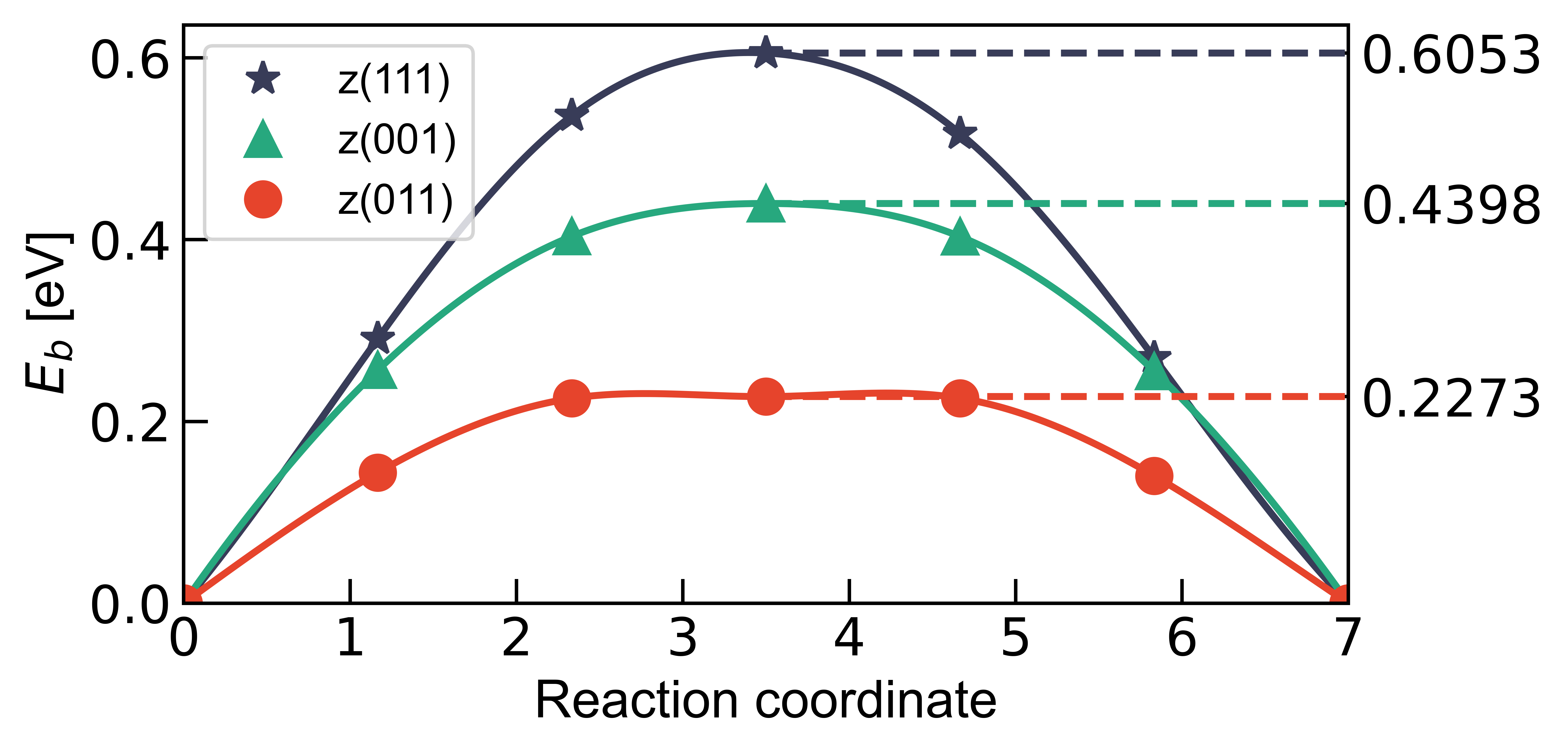
     activation energy (->) =   0.605300 eV
     activation energy (<-) =   0.605300 eV

     image        energy (eV)        error (eV/A)        frozen

         1    -170297.5068071            0.012869            F
         2    -170297.2157836            0.049556            F
         3    -170296.9703486            0.043986            F
         4    -170296.9015067            0.047150            F
         5    -170296.9901551            0.058420            F
         6    -170297.2369477            0.042515            F
         7    -170297.5068071            0.012870            F

     climbing image =  4

     path length          =  5.511 bohr
     inter-image distance =  0.918 bohr
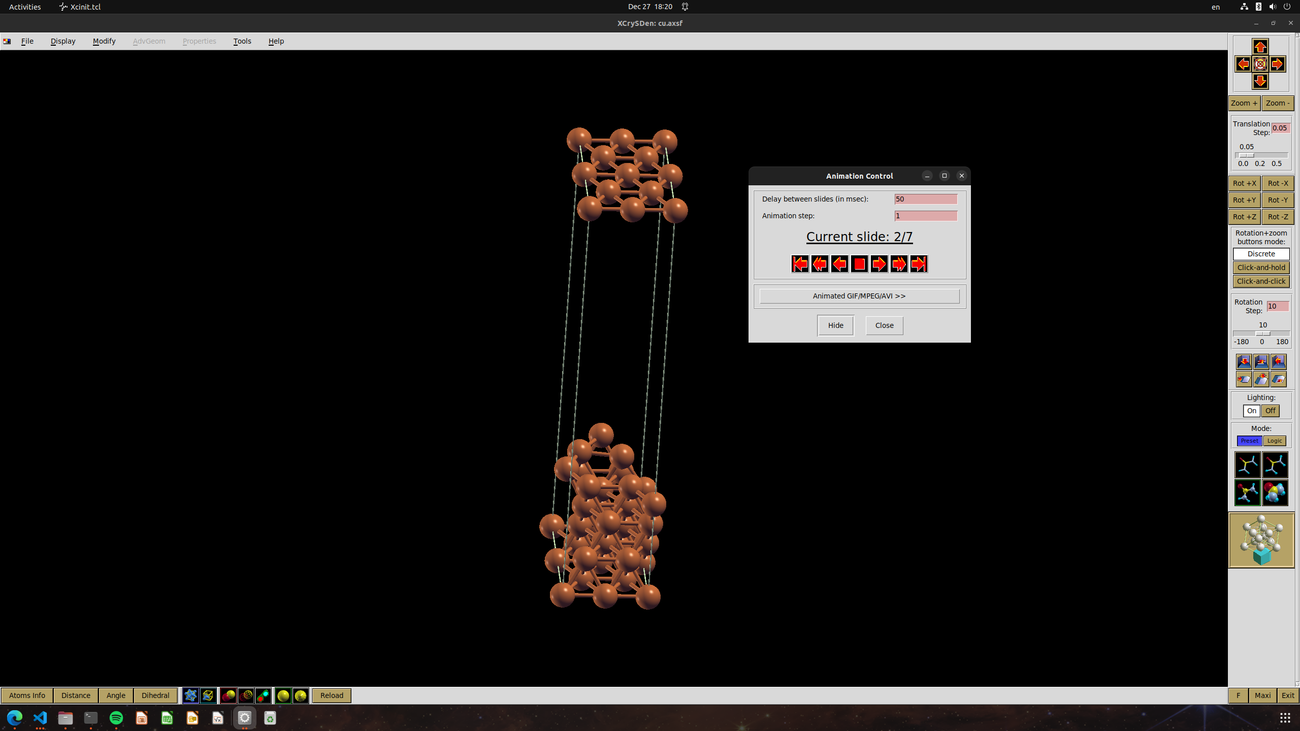
.axsf with xrysden : xcrysden --axsf .axsf 
.crd is something like this, a lot of INTERMEDIATE_IMAGE, can direct copy to neb.in to continue a new calculation based on the present result
FIRST_IMAGE
ATOMIC_POSITIONS (angstrom)
...
INTERMEDIATE_IMAGE
ATOMIC_POSITIONS (angstrom)
...
INTERMEDIATE_IMAGE
ATOMIC_POSITIONS (angstrom)
...
INTERMEDIATE_IMAGE
ATOMIC_POSITIONS (angstrom)
...
INTERMEDIATE_IMAGE
ATOMIC_POSITIONS (angstrom)
...
INTERMEDIATE_IMAGE
ATOMIC_POSITIONS (angstrom)
...
LAST_IMAGE
ATOMIC_POSITIONS (angstrom)
...
.xyz in VESTA, cannot see all the image, only the first can see
.path records the latest result of path calculation, can extract energy (in Ha) and coordinates (seems Bohr, but too many elements, dont know how to convert).
RESTART INFORMATION
       5
      50
       0
NUMBER OF IMAGES
   7
ENERGIES, POSITIONS AND GRADIENTS
Image:    1
    -6258.3179433641
      0.000000000000      0.000000000000      0.000000000000      0.000000000000      0.000000000000      0.000000000000  0  0  0
      2.429384662666     -4.207817256908      0.000000000000      0.000000000000      0.000000000000      0.000000000000  0  0  0
      0.000000000000      8.415634513816      0.000000000000      0.000000000000      0.000000000000      0.000000000000  0  0  0
     -2.429384662666     -4.207817256908      0.000000000000      0.000000000000      0.000000000000      0.000000000000  0  0  0
     -2.429384662666      4.207817256908      0.000000000000      0.000000000000      0.000000000000      0.000000000000  0  0  0
     ...
RESTART INFORMATION is, the present step, total step, and one don’t know. If want to restart and recount the number of step, change the first value to 0.
Image: N below is energy in Ha, but the absolute value may not accord to the value in neb.out. But we only interest in the energy difference, which is in accordance.
Backup all output after NEB finished, before next step!!!
2. CI-NEB
Backup all output after NEB finished, before CI-NEB!!!
use CI_scheme = 'auto' to enable CI calculation
in neb.in
BEGIN
BEGIN_PATH_INPUT
&PATH
  restart_mode      = 'from_scratch'
  string_method     = 'neb'
  nstep_path        = 50      # number of steps for convergence
  ds                = 2.D0    # guess for the diagonal part of the Jacobian matrix
  opt_scheme        = "broyden"
  first_last_opt    = .true.  # optimize the first and last image
  num_of_images     = 7       # number of reaction coordinate
  k_max             = 0.3D0   # elastic variable elastic constants
  k_min             = 0.1D0   # elastic variable elastic constants
  CI_scheme         = "auto"  # use CI ('auto' for using CI, 'no-CI' for no CI)
  path_thr          = 0.1D0   # simulation stops when force error is less than this
  minimum_image     = .true.  # Useful to avoid jumps in the initial reaction path
/
END_PATH_INPUT
...
calculate based on previous NEB calculation
copy all in .crd and paste between:
BEGIN_POSITIONS
...
...
END_POSITIONS
remember to check if there is any atoms need to fixed (like substrate atoms)
Run
mpirun neb.x -i neb.in > neb.out
same as normal NEB
Output
is the same as NEB
3. Migration Energy Barrier
Can use EnergyBarrier to plot the reaction energy barrier 


Leave a Comment