QE PWscf Slab Work Function
Published:
Content
- Atomic Modeling
- 0. structural optimization, kpt convergence, ecut convergence, smearing convergence
- 1. scf
- 2. nscf
- 3. Electronstatic potential postprocessing
- 4. Averge on planes
- 5. Python planar averging
Atomic Modeling
See SlabModeling for slab modeling If pseudo-Hydrogen is using, the workfunciton at H-attached side is not meaningful.
0. structural optimization, kpt convergence, ecut convergence, smearing convergence
Do before any calculation
1. scf
2. nscf
3. Electronstatic potential postprocessing
pp.x
&inputpp
  prefix = '4HSiC'
  outdir = './calout'
  filplot = '4H-SiCslabSi_pot' ! file saving charge density in qe format
  plot_num=  11 ! Differential charge density 9, electrostatic potential (V_bare + V_H) 11, ELF 8
/

! Below no need, only need in 3D file outputing
! &plot
!   nfile = 1
!   iflag = 3 ! 3D ploting
!   output_format = 6 ! Can be read by VESTA
!   fileout = 'charge.prefix.cube' ! Can be read by VESTA
!   e1(1)=1.0,e1(2)=0.0,e1(3)=0.0,
!   e2(1)=0.0,e2(2)=1.0,e2(3)=0.0,
!   e3(1)=0.0,e3(2)=0.0,e3(3)=1.0,
!   x0(1)=1.0,x0(2)=0.0,x0(3)=0.0,
!   nx=101,ny=101,nz=2001
!   ! e1 e2 e3 plotting parallelepiped vectors
!   ! x0 origin of the parallelepiped
!   ! nx ny nz number of points in the parallelepiped
! /
Producing 4H-SiCslabSi_pot
4. Averge on planes
average.x remember Dont use MPI
1
4H-SiCslabSi_potd
1.0
2000
3
5.35255070433784
meaning
- number of 3D-FFT files
- name of 3D-FFT files
- weight of 3D-FFT files
- number of points in the mesh
- direction, defining the planar average (planes perpendicular to this direction)
- macroscopic averege length, in Bohr, usually one unit cell length, not important if do other post-processing with python
Producing avg.dat, including three columns
    position(Bohr) RAW planar    averaged planar
    0.000000000    0.461792073    0.461791837
    0.024566440    0.461820901    0.461790631
    0.049132879    0.461840212    0.461789673
    0.073699319    0.461843995    0.461789148
    0.098265758    0.461831147    0.461789104
    0.122832198    0.461805756    0.461789441
    0.147398638    0.461775773    0.461789942
    0.171965077    0.461750488    0.461790347
    0.196531517    0.461737628    0.461790430
    0.221097957    0.461740962    0.461790069
    0.245664396    0.461759172    0.461789281
    0.270230836    0.461786318    0.461788213
    0.294797275    0.461813735    0.461787095
    0.319363715    0.461832762    0.461786168
    0.343930155    0.461837443    0.461785608
    0.368496594    0.461826349    0.461785476
    0.393063034    0.461802988    0.461785700
    0.417629474    0.461774657    0.461786101
    ...
gnuplot: can also find Fermi level then plot with, found in nscf.out by grep Fermi nscf....out, length can be obtain by the last row first column in tail avg.dat
gnuplot -p -e "plot 'avg.dat' w l, 'avg.dat' u 1:3 w l, [0:49.108312808] 2.3868 w l t 'Fermi level'"

5. Python planar averging
Use PotDistribution
# =========================== need change ========================================
pt1 = 250        # first point dividing outside/inside slab, 0 = not dividing
pt2 = 1800
pt3 = len(xy)
wid1 = 10        # averaging length outside slab
wid2 = 138       # averaging length inside slab, evaluated by period/step
# =========================== need change ========================================
-
ptxdefine the location of the intermediate points, between averaging- normally only three parts are need, first no need averaging (vacuum), second and third have their averaging width defined as
widx
- normally only three parts are need, first no need averaging (vacuum), second and third have their averaging width defined as
-
widxdefine the averaging length, unit is data point inavg.dat
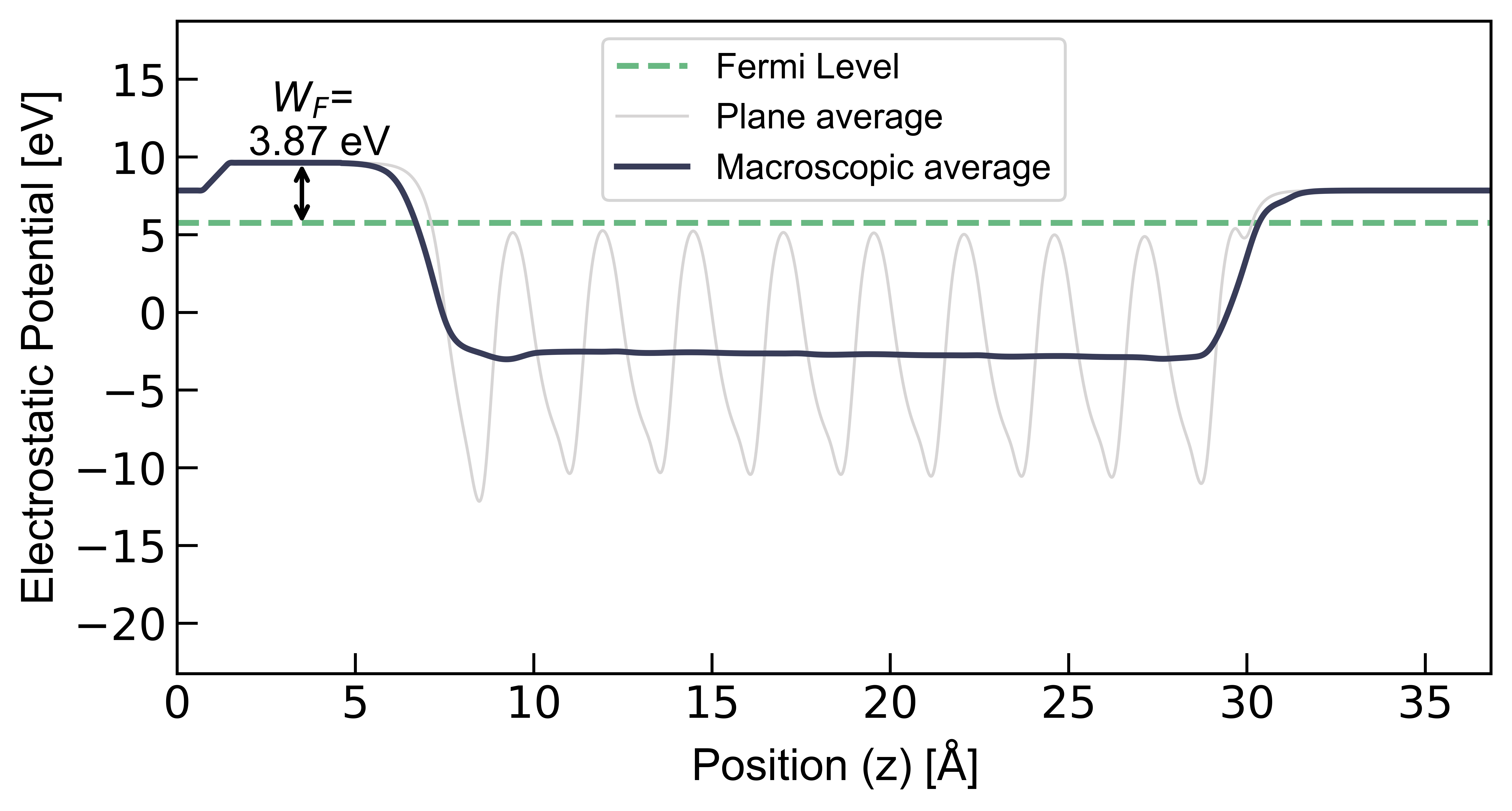
The major purpose of doing averaging is to have a flat interslab potential distribution, by tunning the widx.
A reference value of widx can be obtain by:
- measuring the x difference of the adjacent valleies
- dividing the x difference by variable
step - the integer of this dividing can be reference of
widx


Leave a Comment